In the 1800s, two scientists — Nikola Tesla and Galileo Ferraris —
separately invented their own versions of AC induction motors. Such AC
motors turned out to be reliable alternatives to the DC motors that were
popular at the time. To accurately study induction motors, we must
account for the multiple physics that occur. As today’s example
illustrates, we can include the electromechanical effects in version 5.3
of the COMSOL Multiphysics® software.
Taking a Closer Look at Induction Motors
While both
Nikola Tesla and Galileo Ferraris built early versions of AC induction motors in the 19
th
century, Tesla (a large proponent of AC) is more often credited with
the motor’s invention. This device turned out to be a popular machine,
with future iterations proving to be durable, reliable, and adaptable.
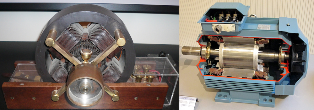 Left: A Tesla induction motor. Image by Ctac — Own work. Licensed under CC BY-SA 3.0, via Wikimedia Commons. Right: A modern three-phase induction motor. Image in the public domain, via Wikimedia Commons.
Engineers can continue to improve these motors by accurately
analyzing their performance, something that requires accounting for all
of the relevant physical effects. To accomplish this, we can couple the
Multibody Dynamics Module and AC/DC Module to analyze electromechanical
effects in a three-phase induction motor. A new example model, added to
the Application Gallery in COMSOL Multiphysics® version 5.3,
demonstrates this functionality.
Using Electromechanical Simulation to Analyze a Three-Phase Induction Motor
We can see all of the parts included in the 3D model of a three-phase
induction motor in the schematic below. We physically model each part
except for the bearings and foundation, which we model as massless
springs.
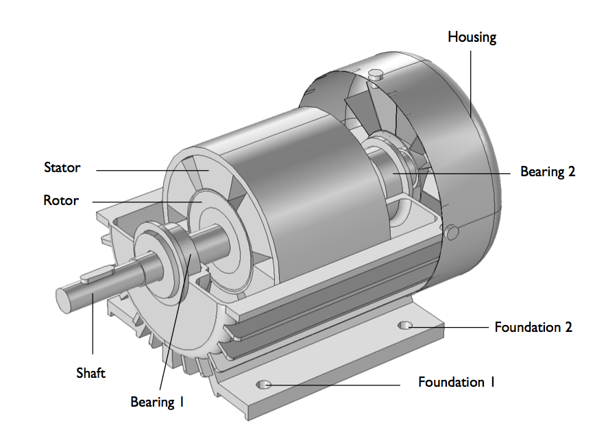 The geometry of the three-phase induction motor housing assembly.
In this example, the stator and rotor are slightly misaligned,
causing the small air gap between them to be asymmetric. As a result of
this asymmetry, vibrations occur in the motor, which can be analyzed
with simulation. To induce eddy currents into the rotor, we rely on the
rotor’s rotation and time-harmonic currents in the stator windings.
Combining Electromagnetics and Multibody Dynamics in COMSOL Multiphysics®
Next, we perform two different studies: a 2D electromagnetics
simulation and a 3D multibody dynamics simulation. In these studies, we
use the
Rotating Machinery interface to account for the motor’s electromagnetic fields and the
Multibody Dynamics interface to simulate the rotor’s motion and housing vibration.
Let’s first discuss the electromagnetic case. For this analysis, we simplify the model to include only three parts:
- Laminated steel stator with zero conductivity
- Rotor with steel inside and aluminum outside
- Asymmetric air gap
This 2D geometry, shown in the cross section below, is a transverse
section of the full 3D geometry. We also apply an alternating current of
60 Hz to the stator winding in this geometry via a
Homogenized Multi-Turn Coil feature that has 2045 turns.
For more information about the geometrical dimensions and electromagnetic model, check out the references in the model documentation.
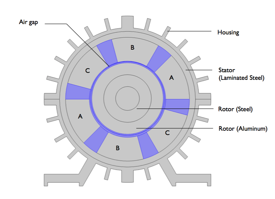 A cross section of a three-phase induction motor model. The three
different coil regions in the stator (labeled A, B, and C) represent the
motor’s three phases.
A cross section of a three-phase induction motor model. The three
different coil regions in the stator (labeled A, B, and C) represent the
motor’s three phases.
Switching gears, let’s explore the multibody dynamics case. This
time, we use the full 3D geometry and model the stator, rotor, and shaft
as rigid, with the rotor rigidly mounted on the shaft. The elastic
hinge joints between the rotor and structural steel housing represent
the bearings, which support the rotor and transmit its forces to the
housing. As for the housing, we assume that it is elastic and use
elastic fixed joints to connect it to the foundation. To compute the
rotor’s angular speed, we use rotational torque, which is calculated as a
function of time.
Using calculations from both of these cases, we run an
electromechanical analysis that couples our electromagnetics and
multibody dynamics simulations. For instance, we add values calculated
with the
Rotating Machinery interface — such as the
electromagnetic forces caused by the stator and rotor misalignment and
the electromagnetic torque — to the rotor and stator in the
Multibody Dynamics interface.
We can find the rotor’s speed by combining these interfaces once
again, transferring the hinge joint’s angular motion computed in the
Multibody Dynamics interface to the
Rotating Machinery interface.
Results for an Electromechanical Analysis of a Three-Phase Induction Motor
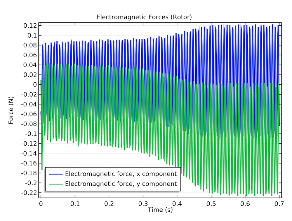
Let’s now take a closer look at the magnetic flux density norm over
time and the rotor’s electromagnetic forces. When calculating these
electromagnetic forces, we observe vibrating forces in the transverse
direction that are caused by the misaligned stator and rotor.
The magnetic flux density norm of the rotor and stator over time
(left) and the rotor’s electromagnetic forces in both the transverse and
axial directions (right).
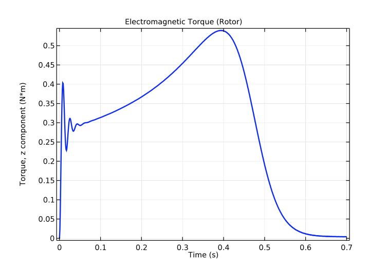
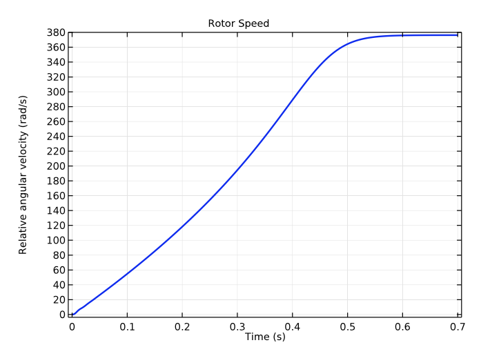
In regards to electromagnetic torque, when the rotor speed equals the
stator electrical frequency, the electromagnetic torque falls to zero
if there is no loading torque on the shaft. The time delay for the rotor
speed to equal the stator electrical frequency is dependent on the
rotor’s inertia. In this case, the rotor takes 0.7 seconds to achieve a
steady-state speed.
The rotor’s electromagnetic torque (left) and angular speed (right) as a function of time.
To find areas of high stress in the motor, we combine our analysis of
the rotor’s velocity with the housing’s von Mises stress distribution.
As indicated in the animation below, the areas near the bearing and
where the housing and foundation connect have the highest stress values.
 The housing’s von Mises stress distribution and the rotor velocity profile.
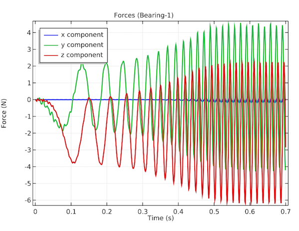
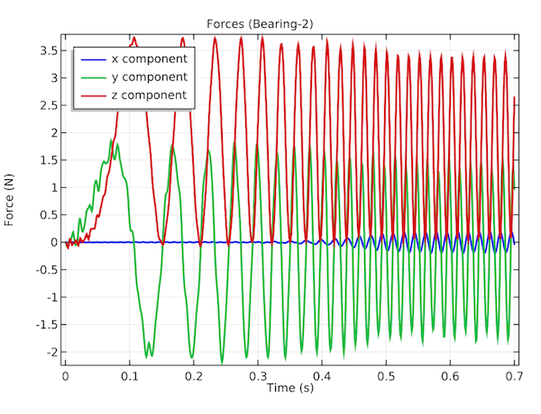
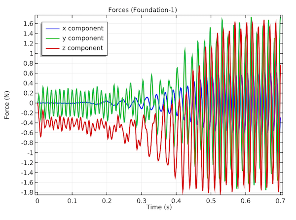
The plots below explore the forces acting on Bearing 1, Bearing 2,
and Foundation 1 as a function of time. These forces travel through the
elastic housing to the motor foundation.
The forces on Bearing 1 (left) and Bearing 2 (middle) in the
transverse and axial directions. The forces at the connection between
the housing and foundation at the location of Foundation 1 (right).
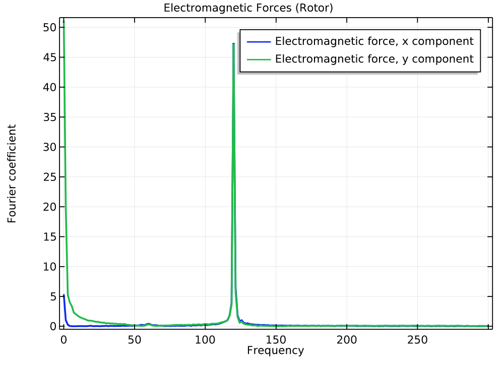
By analyzing the frequency spectrum of the electromagnetic forces, we
can conclude that the frequency is 120 Hz, double the stator electrical
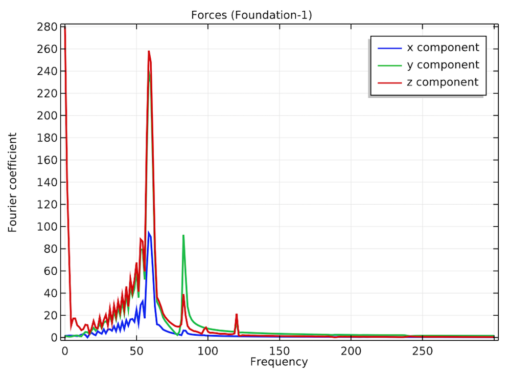
frequency. Despite this, the frequency spectrum plot for the
housing-foundation connection shows a dominant frequency contribution of
around 60 Hz, with a few peaks around 83 Hz — the first natural
frequency of the induction motor’s housing assembly.
The frequency spectrum of the rotor’s electromagnetic forces (left) and forces in the housing-foundation connection (right).
Lastly, let’s examine the rotor’s orbital motion, which results from
the rotor vibrating in the transverse direction, with respect to the
stator. This occurs due to the electromagnetic forces acting on the
rotor in the transverse direction and the finite stiffness of the
bearings supporting the rotor ends. The orbits seen in the following
plot are not concentric due to the rotor’s asymmetric inertia in the
axial direction.
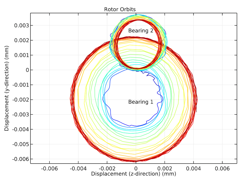 Rotor orbital motion, combining its rotation and vibration, at both bearing locations.
Want to take this electromechanical analysis for a spin? Access the tutorial model with the button below.
Read More About Induction Motors and Electromechanical Simulations
- Take a look at the Multibody Dynamics Release Highlights page to learn more about this and other updates
- Check out these blog posts that combine mechanical and electrical analyses:
- Read about simulating induction motors on the COMSOL Blog: